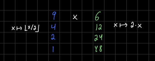
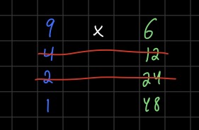
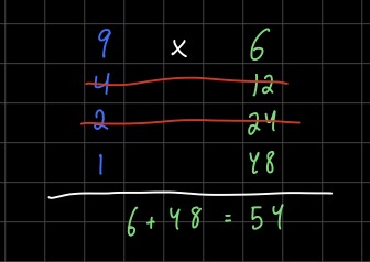
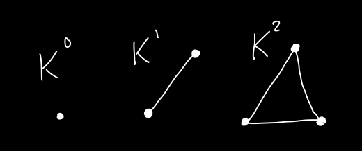
<?xml version="1.0" encoding="utf-8"?><feed xmlns="http://www.w3.org/2005/Atom" xml:lang="en"><generator uri="https://jekyllrb.com/" version="4.4.1">Jekyll</generator><link href="https://eminichiello67.github.io/feed.xml" rel="self" type="application/atom+xml"/><link href="https://eminichiello67.github.io/" rel="alternate" type="text/html" hreflang="en"/><updated>2026-04-18T13:06:24+00:00</updated><id>https://eminichiello67.github.io/feed.xml</id><title type="html">Emilio Minichiello</title><subtitle></subtitle><entry><title type="html">Some Updates</title><link href="https://eminichiello67.github.io/blog/2026/lifeupdate/" rel="alternate" type="text/html" title="Some Updates"/><published>2026-02-17T00:00:00+00:00</published><updated>2026-02-17T00:00:00+00:00</updated><id>https://eminichiello67.github.io/blog/2026/lifeupdate</id><content type="html" xml:base="https://eminichiello67.github.io/blog/2026/lifeupdate/"><![CDATA[<p>Its been a while since I’ve written a blog post here. I wanted to give a little briefer on some updates in my life that I’m quite excited about.</p> <p>First off, my paper <a href="https://arxiv.org/abs/2602.11971">Hypercovers and Differential Geometry</a>, joint with Cheyne Glass, has finally hit the arXiv. I say finally, because I’ve been thinking about hypercovers and the issues this paper addresses since I was just starting out as a graduate student. It revolves around a technical issue that crops up when dealing with model structures on simplicial presheaves. In higher differential geometry–which my thesis <a href="">Higher Diffeology Theory</a> was about, and which my coauthor Cheyne, his advisor Thomas and my advisor Mahmoud have written a bunch of papers about–we want to study manifolds using sheaves of spaces, i.e. simplicial presheaves. We usually deal with the site \((\mathbf{Man}, j_{\text{open}})\) of finite-dimensional smooth manifolds with open covers, or \((\mathbf{Cart}, j_{\text{good}})\), the site of cartesian spaces (spaces diffeomorphic to some \(\mathbb{R}^n\)) with differentiably good open covers. For technical reasons, the latter site is much preferred. So, as is done in my thesis, a big part of higher differential geometry is extracting cocycles from simplicial presheaves on manifolds. Given a site \((\mathcal{C}, j)\), there are two important model structures one can put on the category \(\mathbf{sPre}(\mathcal{C}, j)\) of simplicial presheaves, the Cech projective model structure \(\check{\mathbb{H}}(\mathcal{C}, j)\) and the local projective model structure \(\hat{\mathbb{H}}(\mathcal{C}, j)\). The former has really nice fibrant objects, called \(\infty\)-stacks, and the latter has really nice weak equivalences, called the <strong>local weak equivalences</strong>.</p> <p>The first presents the infinity category of infinity sheaves on \((\mathcal{C}, j)\) and the latter presents the hypercompletion of this infinity category. On certain sites, these two infinity categories are equivalent. We call sites with this property <strong>hypercomplete</strong>. Its been <a href="https://mathoverflow.net/questions/130999/is-the-site-of-smooth-manifolds-hypercomplete">known</a> for a while now that \(\mathbf{Man}\) and \(\mathbf{Cart}\) are hypercomplete, using some material from the latter parts of Lurie’s Higher Topos Theory. However, the more useful thing is to ask when are the Cech and local model categories <strong>equal</strong>. This gives one the best of both worlds: local weak equivalences for weak equivalences and \(\infty\)-stacks for fibrant objects. This paper proves this property for a couple of sites including \(\mathbf{Man}\) and \(\mathbf{Cart}\).</p> <p>This project was close to my heart, as understanding the issues surrounding it led me to more deeply understand sites, leading to my notes <a href="https://arxiv.org/abs/2503.20664">Coverages and Grothendieck Toposes</a>. I think of this paper as the final sort of piece of my extended PhD thesis, which would basically consist of Higher Diffeology Theory, Coverages and Grothendieck Toposes and Hypercovers in Differential Geometry. There is still so much to do, especially in regards to the coverages notes, but I don’t really have much energy for it these days.</p> <p>Instead, I’m really excited about applying abstract math, like category theory, homotopy theory, etc. to discrete mathematical problems. I’ve been learning about a whole ton of really fascinating stuff, like graph homotopy theory, the use of toric varieties in combinatorics, and intersection homology. I really love the mix of abstract methods to solve concrete problems. In this vein, my paper <a href="https://link.springer.com/article/10.1007/s10485-026-09850-6">Thomason-Type Model Structures on Simplicial Complexes and Graphs</a> has just been published by Applied Categorical Structures! In it, I prove that you can transfer the classical model structure on simplicial sets to simplicial complexes, reflexive graphs and loop graphs, leading to a whole sequence of Quillen equivalences, using a similar method that Thomason used for his model structure on \(\mathbf{Cat}\), and I elaborate on some properties of these model categories. This provides some more details on <a href="https://intlpress.com/site/pub/files/_fulltext/journals/hha/2017/0019/0002/HHA-2017-0019-0002-a010.pdf">Matsushita’s construction</a> of a model structure on loop graphs.</p> <p>Speaking of graph homotopy and homology, I made some updates to my list of papers on the subject at the discretepapers tab. There’s an endless list of fascinating papers to read on this subject, but hopefully soon I’ll have most of the big ones listed there.</p> <p>On the teaching side, I’m teaching a really cool course: introduction to category theory at CUNY CityTech. This is the first time a course like this has been taught to undergraduates there, and I’m having loads of fun. I’m aiming to first introduce some of the basic discrete mathematical structures: sets, posets, monoids, graphs and simplicial complexes, and then introduce the basic ideas of category theory through these examples. I’ll try and report back my thoughts on this later in the semester.</p> <p>I’ve also become co-organizer of the NYC Category Theory seminar, which has also changed from a 7pm time to a 2pm time on Wednesdays, which is way more convenient. We’ve got a really great lineup this semester, which you can check out <a href="https://www.sci.brooklyn.cuny.edu/~noson/Seminar/">here</a>.</p> <p>I’ll be giving a talk at a conference <a href="https://sites.google.com/view/hhgraphs">Homotopy and Homology in Graphs</a> in Switzerland at EPFL in September about my Thomason-Type model structures paper. I’m really excited about this, shoot me an email if you’ll be attending as well!</p> <p>I’ll probably go to another conference during the summer, but there are so many good choices, I’m not sure yet which I’ll choose.</p> <p>I’m super excited for this year, but I’m not going to lie, entering a new field feels really daunting. I’ve been thinking about higher differential geometry for my whole PhD. Now I have to retrain myself to think more like a combinatorialist. Its probably a bad idea to switch fields this early in one’s math career, but I’m confident that it’ll be okay, the upside being that this new area (abstract math applied to discrete math) has loads of fascinating things going on. In one direction I’m in awe of the fast-growing theory of algebraic topology being applied to graphs. Check out my discretepapers tab if you want to see a bunch of cool papers, and in another, I’m working with Ben Bumpus on some more stuff related to category theory, graph theory and algorithms. Hopefully more on that soon! I’ve been learning a lot of graph theory, and especially about different graph classes. These graph classes are really fascinating, and studying them makes me feel like there could be really interesting invariants one could extract from them. Like I want to treat a whole graph class of a certain kind as a single mathematical object (maybe like a spectrum in homotopy theory). Anyway, this post is just some rambling, maybe I’ll ramble some more soon.</p>]]></content><author><name></name></author><category term="math"/><summary type="html"><![CDATA[updates on life]]></summary></entry><entry><title type="html">Papers on Graph Homotopy Theory</title><link href="https://eminichiello67.github.io/blog/2025/graphhomotopytheory/" rel="alternate" type="text/html" title="Papers on Graph Homotopy Theory"/><published>2025-09-01T00:00:00+00:00</published><updated>2025-09-01T00:00:00+00:00</updated><id>https://eminichiello67.github.io/blog/2025/graphhomotopytheory</id><content type="html" xml:base="https://eminichiello67.github.io/blog/2025/graphhomotopytheory/"><![CDATA[<p>Here we list some papers in the burgeoning subject of discrete homotopy theory, which considers applications of homotopy theory to discrete mathematics. The largest branch of this subject is graph homotopy theory, which itself splits into two sub-pieces: the \(\times\)-homotopy theory and the \(A\)-homotopy theory, which can be thought of as the simplicial graph homotopy theory and the cubical graph homotopy theory, respectively. This page will be updated occasionally</p> <hr/> <h2 id="a-homotopy-theory">A-Homotopy Theory</h2> <details> <summary>(2001) <strong>Foundations of a Connectivity Theory for Simplicial Complexes</strong> by Hélène Barcelo, Xenia Kramer, Reinhard Laubenbacher and Christopher Weaver.</summary> <script id="MathJax-script" async="" src="https://cdn.jsdelivr.net/npm/mathjax@4/tex-mml-chtml.js"></script> <ul> <li>Advances in Applied Mathematics 26, no. 2 (2001): 97–128. (<a href="https://doi.org/10.1006/aama.2000.0710">link</a>) <br/></li> <li>I consider this to be the first paper in A-homotopy theory, even though it is based off of papers by Atkins and his students, inspired by work in the social sciences on social dynamics, which are about what he calls Q-analysis of simplicial complexes. In this paper, Barcelo et al really get to work putting Atkins' idea on a a rigorous footing.</li> <li>They define the A-homotopy group \(A^q_n(\Delta, x_0)\) of a simplicial complex.</li> <li>They associate to every simplicial complex \(\Delta\) a \(q\)-conectivity graph \(\Gamma^q(\Delta)\), whose vertices are the simplices of \(\Delta\) of dimension \(\geq q\) and whose edges connect those simplices which share a \(q\)-face. They define the \(A\)-homotopy groups of a graph \(A_n(G, x_0)\) such that \(A_n(\Gamma^q(\Delta), x_0) \cong A^q_n(\Delta, x_0)\).</li> <li>They show that the \(A\)-fundamental group \(A^q_1(\Delta, x_0) \) can be computed easily by taking the \(q\)-connectivity graph \(\Gamma^q(\Delta)\) and filling in all 3 and 4-cycles with a 2-cell, and taking the usual fundamental group of the resulting CW complex.</li> <li>They prove a Seifert-Van Kampen type theorem for the \(A\)-fundamental group.</li> </ul> </details> <details> <summary> (2005) <strong>Perspectives on A-Homotopy Theory and Its Applications</strong> by Hélène Barcelo, and Reinhard Laubenbacher. </summary> <script id="MathJax-script" async="" src="https://cdn.jsdelivr.net/npm/mathjax@4/tex-mml-chtml.js"></script> <ul> <li>Discrete Mathematics, Formal Power Series and Algebraic Combinatorics 2002 (FPSAC’02), vol. 298, no. 1 (2005): 39–61. (<a href="https://doi.org/10.1016/j.disc.2004.03.016.">link</a>) </li> <li> Really wonderful paper that gives a whole bunch of applications and relationships of \(A\)-homotopy theory to combinatorics. Barcelo and Laubenbacher show that \(A\)-homotopy theory shows up in the work of several combinatorialists: <ul> <li>in the <a href="https://doi.org/10.1016/0095-8956(73)90005-1">work of Maurer (1973)</a> on matroids. In particular Maurer proves that if \(M\) is a matroid, and \(\mathcal{B}(M) \) is the basis graph of \(M\), then \(\mathcal{B}(M)\) has \(A_1(\mathcal{B}(M) = 0 \).</li> <li>in the <a href="https://doi.org/10.1007/BF01896190">work of Lovasz (1977)</a> on \(k\)-fold partitions of \(k\)-connected graphs,</li> <li>in the <a href="https://web.math.pmf.unizg.hr/glasnik/18.1/18101.pdf">work of Malle (1983)</a>, who proves that if \(G\) is a graph, then \(A_1(G) = 0\) if and only if every cycle in \(G\) has a pseudoplanar net in \(G\).</li> <li> in the work of Babson and Bjorner, but published later by <a href="">Barcelo-Severs-White (2011)</a> as Theorem 3.1. The \(k\)-equal arrangement, \(A_{n,k} \) is the collection of all subspaces of \( \mathbb{R}^{n+1} \) given by \(x_{i_1} = x_{i_2} = \dots = x_{i_k}\) over all indices \({i_1, \dots , i_k} \subseteq [ n + 1]\), with the relation \(\sum_{i=1}^{n+1} x_i = 0 \). They prove that if \(U(A_{n,k}) \) denotes the complement of \(A_{n,k}\) in \(\mathbb{R}^{n+1} \), then \(\pi_1(U(A_{n,k})) \cong A_1^{n - k + 1}(\Delta(B_n)) \), where \(\Delta(B_n) \) is the order complex of the Boolean lattice \(B_n = \{0,1\}^n \). </li> </ul> </li> </ul> </details> <details> <summary>(2006) <strong>Homotopy Theory of Graphs</strong> by Eric Babson, Hélène Barcelo, Mark Longueville, and Reinhard Laubenbacher.</summary> <script id="MathJax-script" async="" src="https://cdn.jsdelivr.net/npm/mathjax@4/tex-mml-chtml.js"></script> <ul> <li>J. Algebraic Comb. 24, no. 1 (2006): 31–44. (<a href="https://doi.org/10.1007/s10801-006-9100-0">link</a>)</li> <li>One of the key results of the 2001 Foundations paper computes the \(A\)-fundamental group of a graph \(G\) in terms of the usual fundamental group of a related space \(X_G \) obtained by filling in the 3 and 4 cycles with 2-cells. This paper addresses the question of this can be achieved for the higher \(A\)-homotopy groups. </li> <li> They define the loop graph \(\Omega G \) of a graph \(G \) and prove that \( A_{n+1}(G) \cong A_n(\Omega G) \) for \(n \geq 0 \).</li> <li> Given a graph \(G \), they construct a cubical set \(N_1(G) \) (which they denote \(M_*(G) \), but we will use the notation from <a href="https://doi.org/10.1112/S0010437X24007486.">Kapulkin-Carranza (2024)</a>) and prove that if a certain cubical approximation conjecture holds (and note that as of this writing, this conjecture is still open) then \(\pi_n(N_1(G)) \cong A_n(G) \) for all \(n \geq 1 \). <ul> <li>Note that the above result was later proven in <a href="https://doi.org/10.1112/S0010437X24007486.">Kapulkin-Carranza (2024)</a>, using abstract homotopy theory, entirely avoiding having to prove the cubical approximation conjecture.</li> </ul> </li> </ul> </details> <details> <summary>(2014) <strong> Discrete Homology Theory for Metric Spaces</strong> by Hélène Barcelo, Valerio Capraro, and Jacob A. White. </summary> <script id="MathJax-script" async="" src="https://cdn.jsdelivr.net/npm/mathjax@4/tex-mml-chtml.js"></script> <ul> <li>Bulletin of the London Mathematical Society 46, no. 5: 889–905. (<a href="https://doi.org/10.1112/blms/bdu043">link</a>) </li> <li>Develops a notion of discrete homology for metric spaces that satisfies a discrete form of the Eilenberg-Steenrod axioms.</li> <li>Unfortunately, the Mayer-Vietoris theorem proven here is not as useful as one might think for A-homotopy theory. In the context of A-homotopy theory, the kind of cover needed for excision and Mayer-Vietoris would be a discrete cover, which is a cover of a graph by subgraphs such that every nondegenerate singular cube \(f : Q_n \to G \) factors through one of the subgraphs. In practice this cannot be checked, as there is an enormous amount of nondegenerate singular cubes of high dimensions.</li> </ul> </details> <details> <summary>(2019) <strong>Discrete Cubical and Path Homologies of Graphs</strong> by Hélène Barcelo, Curtis Greene, Abdul Salam Jarrah, and Volkmar Welker.</summary> <script id="MathJax-script" async="" src="https://cdn.jsdelivr.net/npm/mathjax@4/tex-mml-chtml.js"></script> <ul> <li>Algebraic Combinatorics 2, no. 3 (2019): 417–37. (<a href="https://doi.org/10.5802/alco.49">link</a>) </li> <li>Specializes the definition of discrete homology for metric spaces from <a href="https://doi.org/10.1112/blms/bdu043">Barcelo-Capraro-White (2014)</a> to graphs, calls it discrete cubical homology. We will use the notation \(H_n^\square(G) \) for these homology groups of a graph \(G \).</li> <li>Proves that all trees are \(A\)-contractible</li> <li>Proves that all hypercubes \(Q_n\) are \(A\)-contractible</li> <li>Proves that all chordal graphs are cubical acyclic, i.e. if \(G\) is chordal, then \(H_n^\square(G) = 0 \) for all \(n \geq 1\).</li> <li>Proves that complete bipartite graphs are cubical acyclic</li> <li>Proves that discrete cubical homology and path homology do not always agree. Also shows that the Greene Sphere graph has nontrivial \(H_2^\square\) (Theorem 6.1).</li> </ul> </details> <details> <summary>(2020) <strong>Higher Discrete Homotopy Groups of Graphs</strong> by Bob Lutz.</summary> <script id="MathJax-script" async="" src="https://cdn.jsdelivr.net/npm/mathjax@4/tex-mml-chtml.js"></script> <ul> <li> Algebraic Combinatorics 4, no. 1 (2021): 69–88. (<a href="https://doi.org/10.5802/alco.151.">link</a>) </li> <li> The main theorem of this paper is the following: Suppose that \(G \) is a graph without 3 or 4-cycles. Then \(A_n(G,x) = 0 \) for every \(n \geq 2 \) and \(x \in G \).</li> <li> This result is the homotopy group analogue of a similar theorem proved by Barcelo, Greene, Jarrah and Welker for cubical homology.</li> <li> This result can nowadays be proved using the covering space theory developed in [Kapulkin-Mavinkurve (2025)](https://doi.org/10.1016/j.aam.2024.102838). Indeed, a graph with no 3 or 4-cycles has a forest for an universal cover. Kapulkin-Mavinkurve prove that the universal cover induces an isomorphism on higher homotopy groups, proving the theorem, as forests can easily be shown to have zero higher A-homotopy groups.</li> </ul> </details> <details> <summary>(2021) <strong>On the Vanishing of Discrete Singular Cubical Homology for Graphs</strong> by Hélène Barcelo, Curtis Greene, Abdul Salam Jarrah, and Volkmar Welker.</summary> <script id="MathJax-script" async="" src="https://cdn.jsdelivr.net/npm/mathjax@4/tex-mml-chtml.js"></script> <ul> <li>SIAM Journal on Discrete Mathematics, 2021 (<a href="https://epubs.siam.org/doi/abs/10.1137/20M1338484">link</a>) </li> <li>This paper is about a very impressive result that says that if a graph \(G\) has no 3 or 4-cycles, then its higher discrete cubical homology vanishes: \(H_n^{\square}(G) = 0\) for \(n \geq 2\). The proof is quite involved. The idea is to lift a cube to the universal cover, subdivide it, and then map it back down to the graph, crafting a homotopy equivalence between the singular n-cube chain complex and a subcomplex consisting of cubes whose image has cardinality less than 2.</li> </ul> </details> <details> <summary>(2024) <strong>Cubical Setting for Discrete Homotopy Theory, Revisited</strong> by Krysztof Kapulkin and Daniel Carranza</summary> <script id="MathJax-script" async="" src="https://cdn.jsdelivr.net/npm/mathjax@4/tex-mml-chtml.js"></script> <ul> <li>Compositio Mathematica 160, no. 12 (2024): 2856–903. (<a href="https://doi.org/10.1112/S0010437X24007486.">link</a>) </li> <li>This paper proved the following conjecture from [Babson, Barcelo,Longueville and Laubenbacher (2006)](https://doi.org/10.1007/s10801-006-9100-0): Given a graph \(G\), there exists a topological space \(X_G\) such that \(A_n(G) \cong \pi_n(X_G) \) for all \(n \geq 0\). </li> <li>Kapulkin-Carranza prove this by crafting a cubical nerve functor from graphs to cubical sets. After some very involved calculations, they show that this cubical nerve is a cubical Kan complex, and can transfer a category of fibrations structure over to graphs, and prove that the homotopy groups of this cubical Kan complex are precisely the A-homotopy groups. This gives a powerful tool to study the A-homotopy groups of a graph, but this cubical nerve functor is still very hard to study. Even for the simplest graphs, it is wildly huge, with nondegenerate cells in every dimension (consider the map \(Q_n \to K_2 \) that takes the logical sum 0 + 0 = 1 + 1 = 0, 0 + 1 = 1 + 0 = 1, this is a nondegenerate graph map that is nondegenerate in every dimension).</li> </ul> </details> <details> <summary>(2025) <strong>The Fundamental Group in Discrete Homotopy Theory</strong> by Krysztof Kapulkin and Udit Mavinkurve</summary> <script id="MathJax-script" async="" src="https://cdn.jsdelivr.net/npm/mathjax@4/tex-mml-chtml.js"></script> <ul> <li>Advances in Applied Mathematics 164 (March 2025): 102838 (<a href="https://doi.org/10.1016/j.aam.2024.102838.">link</a>) </li> <li>Gives a very nice account of covering theory for graphs, improving upon previous accounts, and crafting a universal cover for graphs that may have 3 or 4-cycles. Is able to construct for any finitely presented group A a graph G whose fundamental group is \(\pi_1(G) = A \). However, it is unknown what the higher homotopy groups of this construction are.</li> </ul> </details> <details> <summary>(2025) <strong>The Lifting Properties of A-Homotopy Theory</strong> by Rachel Morrill</summary> <script id="MathJax-script" async="" src="https://cdn.jsdelivr.net/npm/mathjax@4/tex-mml-chtml.js"></script> <ul> <li>arXiv (<a href="https://doi.org/10.48550/arXiv.1904.12065">link</a>) </li> </ul> </details> <details> <summary>(2025) <strong>Mapping Fiber, Loop and Suspension Graphs in Naive Discrete Homotopy Theory</strong> by Rachel Morrill</summary> <script id="MathJax-script" async="" src="https://cdn.jsdelivr.net/npm/mathjax@4/tex-mml-chtml.js"></script> <ul> <li>arXiv (<a href="https://doi.org/10.48550/arXiv.2402.15714">link</a>) </li> </ul> </details> <hr/> <h2 id="x-homotopy-theory">X-Homotopy Theory</h2> <details> <summary>(2009) <strong>Hom complexes and homotopy theory in the category of graphs </strong> by Anton Dochtermann</summary> <script id="MathJax-script" async="" src="https://cdn.jsdelivr.net/npm/mathjax@4/tex-mml-chtml.js"></script> <ul> <li>European Journal of Combinatorics 30.2 (2009): 490-509 (<a href="https://doi.org/10.1016/j.ejc.2008.04.009">link</a>) </li> </ul> </details> <details> <summary>(2009) <strong>Homotopy groups of Hom complexes of graphs</strong> by Anton Dochtermann</summary> <script id="MathJax-script" async="" src="https://cdn.jsdelivr.net/npm/mathjax@4/tex-mml-chtml.js"></script> <ul> <li> Journal of Combinatorial Theory, Series A 116.1 (2009): 180-194. (<a href="https://doi.org/10.1016/j.jcta.2008.06.001">link</a>) </li> </ul> </details> <details> <summary>(2017) <strong>Box Complexes and Homotopy Theory of Graphs</strong> by Takahiro Matsushita</summary> <script id="MathJax-script" async="" src="https://cdn.jsdelivr.net/npm/mathjax@4/tex-mml-chtml.js"></script> <ul> <li>Homology, Homotopy and Applications, vol. 19(2), 2017, pp.175–197 (<a href="http://dx.doi.org/10.4310/HHA.2017.v19.n2.a10">link</a>) </li> </ul> </details> <details> <summary>(2025) <strong>Thomason-Type Model Structures on Simplicial Complexes and Graphs</strong> by Emilio Minichiello</summary> <script id="MathJax-script" async="" src="https://cdn.jsdelivr.net/npm/mathjax@4/tex-mml-chtml.js"></script> <ul> <li>arXiv (<a href="https://arxiv.org/abs/2508.08195">link</a>) </li> </ul> </details> <hr/> <h2 id="path-homology">Path Homology</h2> <details> <summary>(2012) <strong>Homologies of Path Complexes and Digraphs</strong> by Alexander Grigor'yan, Yong Lin, Yuri Muranov, Shing-Tung Yau</summary> <script id="MathJax-script" async="" src="https://cdn.jsdelivr.net/npm/mathjax@4/tex-mml-chtml.js"></script> <ul> <li>arXiv (<a href="https://arxiv.org/abs/1207.2834">link</a>) </li> </ul> </details> <h2 id="čech-closure-spaces-and-pseudotopological-spaces">Čech Closure Spaces and Pseudotopological Spaces</h2> <details> <summary>(2021) <strong>Eilenberg-Steenrod homology and cohomology theories for Čech's closure spaces</strong> by Peter Bubenik and Nikola Milićevic</summary> <script id="MathJax-script" async="" src="https://cdn.jsdelivr.net/npm/mathjax@4/tex-mml-chtml.js"></script> <ul> <li>arXiv (<a href="https://arxiv.org/abs/2112.13421">link</a>) </li> </ul> </details> <details> <summary>(2021) <strong>Homotopy, homology, and persistent homology using closure spaces</strong> by Peter Bubenik and Nikola Milićevic</summary> <script id="MathJax-script" async="" src="https://cdn.jsdelivr.net/npm/mathjax@4/tex-mml-chtml.js"></script> <ul> <li> J. Appl. Comput. Topol. 8 (2024), no. 3, 579-641 (<a href="https://doi.org/10.1007/s41468-024-00183-8">link</a>) </li> </ul> </details>]]></content><author><name></name></author><category term="math"/><category term="graphs,"/><category term="homotopy"/><category term="theory"/><summary type="html"><![CDATA[A repository of papers]]></summary></entry><entry><title type="html">Duplation-Mediation Multiplication</title><link href="https://eminichiello67.github.io/blog/2024/duplation-multiplication/" rel="alternate" type="text/html" title="Duplation-Mediation Multiplication"/><published>2024-11-16T00:00:00+00:00</published><updated>2024-11-16T00:00:00+00:00</updated><id>https://eminichiello67.github.io/blog/2024/duplation-multiplication</id><content type="html" xml:base="https://eminichiello67.github.io/blog/2024/duplation-multiplication/"><![CDATA[<p>I’ve been learning about algorithms lately, and I learned about an alternative algorithm for multiplication. Doubtless most readers here will probably have heard of this algorithm, its super well-known, but I had never heard of it before, and I had a surprisingly hard time understanding why it worked. So I’m gonna write a short, fun little blog post about this.</p> <p>The algorithm is called by many names, one of which is Russian peasant multiplication[^1]. I think this is a pretty shitty name, so I’m just going to call it <strong>duplation-mediation multiplication</strong>. The reason for that name should become apparent shortly. This algorithm is super old, it was used by the ancient Egyptians for example, and I think it is actually easier to do than the method of multiplying that I learned in elementary schoool.</p> <p>The algorithm goes like this. Suppose we want to multiply \(9 \times 6\). We write them side-by-side and then keep dividing \(9\) by \(2\), throwing away any remainder, until we get to \(1\). On the other side, we keep multiplying \(6\) by \(2\). The operation of multiplying by \(2\) is called <strong>duplation</strong> and the operation of dividing by \(2\) and throwing away the remainder is called <strong>mediation</strong>, hence the name of the algorithm. In other words, mediation is the operation \(x \mapsto \lfloor x/2 \rfloor\) and duplation is \(x \mapsto 2x\).</p> <div align="center"> <figure> <p><img src="../../../assets/img/posts/duplation/pic1.jpg" alt="Step 1 of Duplation-Mediation" width="500"/></p> <figcaption>Figure 1: Step 1 of Duplation-Mediation</figcaption> </figure> </div> <p>Okay, now the next step is to cross out all of the rows in which the left hand number is even.</p> <div align="center"> <figure> <p><img src="../../../assets/img/posts/duplation/pic2.jpg" alt="Step 2 of Duplation-Mediation" width="400"/></p> <figcaption>Figure 2: Step 2 of Duplation-Mediation</figcaption> </figure> </div> <p>Finally we add up the numbers on the right hand column.</p> <div align="center"> <figure> <p><img src="../../../assets/img/posts/duplation/pic3.jpg" alt="Step 3 of Duplation-Mediation" width="400"/></p> <figcaption>Figure 3: Step 3 of Duplation-Mediation</figcaption> </figure> </div> <p>Like magic, we get the right answer \(9 \times 6 = 54\)! When I first saw this I was kind of baffled. It was clear to me that something was going on with converting the numbers to binary, but I wasn’t quite sure what was happening.</p> <p>The first thing I noticed is that if we convert our numbers from decimal to binary, then the operation of mediation \(x \mapsto \lfloor x/2 \rfloor\) is the same thing as taking the right-shift in binary. In other words, if we consider \(9\) in binary, which is \([9]_2 = 1001\), then \([\lfloor 9/2 \rfloor]_2 = [4]_2 = 100\). Similarly, duplation \(x \mapsto 2x\) is the same thing as left-shift in binary, for example since \([6]_2 = 110\) and \([2 \times 6]_2 = [12]_2 = 1100\). So that was interesting, but what was up with the crossing out part?</p> <p>Well what helped me understand this the most was by writing \(9\) in its binary expansion. \(9 = 2^3 + 2^0 = 8 + 1\). So \(9 \times 6 = (2^3 + 2^0) \times 6 = 2^0 \times 6 + 2^3 \times 6\). In the pictures above, we have \(2^0 \times 6 = 6\) appearing at the top, and \(2^3 \times 6 = 48\) appearing at the bottom. In other words, we crossed out the other two rows because \(2^1\) and \(2^2\) don’t appear in the binary expansion of \(9\)!</p> <p>But why does the left hand column give the binary expansion of \(9\)? Well, what is the binary expansion of \(9\)? It is \(1001\). The rightmost digit is \(1\) because \(9\) is odd, i.e. \(9 \text{ mod } 2 = 1\). The next digit can be obtained by looking at the right shift of \(1001\), which is \(100\), which in decimal is \(\lfloor 9/2 \rfloor = 4\). Since this number is even, the rightmost digit is \(0\). Doing this again we have \(\lfloor 4/2 \rfloor = 2 = 10\), and \(\lfloor 2 \rfloor = 1\) in decimal and binary. In other words, you can easily obtain the binary representation of any integer by just keep on dividing it in half and seeing whether it is even or odd.</p> <p>Hopefully this little post brought you some joy and taught you something new. It should be said that this algorithm is technically not any more efficient than the usual way of multiplying, they are both \(\mathcal{O}(n^2)\). But I find multiplying and dividing by \(2\) mentally easier, and then at the end we just sum them up.</p> <hr/> <p>[^1] According to Wikipedia, it also goes by ancient Egyptian multiplication, Ethiopian multiplication, Russian multiplication and peasant multiplication.</p>]]></content><author><name></name></author><category term="math"/><category term="fun,"/><category term="algorithms"/><summary type="html"><![CDATA[Let's discuss an alternative algorithm for multiplication.]]></summary></entry><entry><title type="html">Pushouts along monomorphisms.</title><link href="https://eminichiello67.github.io/blog/2024/adhesivecategories/" rel="alternate" type="text/html" title="Pushouts along monomorphisms."/><published>2024-11-14T00:00:00+00:00</published><updated>2024-11-14T00:00:00+00:00</updated><id>https://eminichiello67.github.io/blog/2024/adhesivecategories</id><content type="html" xml:base="https://eminichiello67.github.io/blog/2024/adhesivecategories/"><![CDATA[<p>Continuing on with the previous blog posts about categories of simple graphs, let us talk about a special class of categories, called <strong>adhesive categories</strong> and show that \(\mathsf{rGrph}\) belongs to this class.</p> <p>Let’s start with the definition: A category \(\mathcal{C}\) is <strong>adhesive</strong> if</p> <ul> <li>it has pullbacks, and</li> <li>pushouts along monomorphisms<sup id="fnref:1"><a href="#fn:1" class="footnote" rel="footnote" role="doc-noteref">1</a></sup> exist and are Van Kampen.</li> </ul> <p>Okay, so this might seem a little weird at first glance. What exactly does it mean for pushouts along monomorphisms to be Van Kampen? What does that have to do with graphs? All in due time, be patient!</p> <p>First, let’s discuss Van Kampen colimits. This is a topic that really deserves a blog post of its own, so I’ll only give some basic details. We say a diagram \(d: I \to \mathcal{C}\) has a <strong>Van Kampen</strong> colimit if the colimit of \(d\) exists and there is an equivalence \(\mathcal{C}_{/\text{colim}_i \, d(i)} \simeq \lim_i \mathcal{C}_{/d(i)},\) where on the right hand side we have a pseudolimit.</p> <p>The big idea here is: a diagram’s colimit is Van Kampen if you can “get the pieces back after you glued them together.”</p> <p>Both the equivalence above and that vague statement might leave you feeling angry, and I understand. Here’s a much more concrete way to think about this in the case when the diagram is a pushout.</p> <p>So suppose we have a diagram \(Y_0 \xleftarrow{g_0} Y_1 \xrightarrow{g_1} Y_2\) and let \(Y = Y_0 +_{Y_1} Y_2\) be its colimit, i.e. pushout. Suppose we have a map \(\alpha : X \to Y\), and we take pullbacks </p> <iframe class="quiver-embed" src="https://q.uiver.app/#q=WzAsNixbMSwxLCJZIl0sWzEsMCwiWCJdLFswLDEsIllfMCJdLFsyLDEsIllfMiJdLFswLDAsIlhfMCJdLFsyLDAsIlhfMiJdLFsxLDAsIlxcYWxwaGEiLDJdLFsyLDAsIlxcbGFtYmRhXzAiLDJdLFszLDAsIlxcbGFtYmRhXzIiXSxbNCwyLCJcXGFscGhhXzAiLDJdLFs0LDEsIlxcc2lnbWFfMCJdLFs1LDMsIlxcYWxwaGFfMiJdLFs1LDEsIlxcc2lnbWFfMiIsMl0sWzQsMCwiIiwwLHsic3R5bGUiOnsibmFtZSI6ImNvcm5lciJ9fV0sWzUsMCwiIiwwLHsic3R5bGUiOnsibmFtZSI6ImNvcm5lciJ9fV1d&amp;embed" width="432" height="304" style="border-radius: 8px; border: none;"></iframe> <p>This is like “breaking X into pieces.” We then take two more pullbacks to obtain a big commutative cube </p> <iframe class="quiver-embed" src="https://q.uiver.app/#q=WzAsOCxbMiwzLCJZIl0sWzIsMSwiWCJdLFswLDMsIllfMCJdLFszLDIsIllfMiJdLFswLDEsIlhfMCJdLFszLDAsIlhfMiJdLFsxLDAsIlhfMSJdLFsxLDIsIllfMSJdLFsxLDAsIlxcYWxwaGEiLDEseyJsYWJlbF9wb3NpdGlvbiI6MzB9XSxbMiwwLCJcXGxhbWJkYV8wIiwxXSxbMywwLCJcXGxhbWJkYV8yIiwxXSxbNCwyLCJcXGFscGhhXzAiLDIseyJsYWJlbF9wb3NpdGlvbiI6MzB9XSxbNCwxLCJcXHNpZ21hXzAiLDEseyJsYWJlbF9wb3NpdGlvbiI6NzB9XSxbNSwzLCJcXGFscGhhXzIiXSxbNSwxLCJcXHNpZ21hXzIiLDFdLFs0LDAsIiIsMCx7InN0eWxlIjp7Im5hbWUiOiJjb3JuZXIifX1dLFs2LDQsImZfMCIsMl0sWzYsNSwiZl8xIl0sWzcsMiwiZ18wIiwyXSxbNywzLCJnXzEiLDAseyJsYWJlbF9wb3NpdGlvbiI6MzB9XSxbNiw3LCJcXGFscGhhXzEiLDEseyJsYWJlbF9wb3NpdGlvbiI6NzB9XSxbNiwzLCIiLDEseyJzdHlsZSI6eyJuYW1lIjoiY29ybmVyIn19XSxbNiwxMSwiIiwxLHsibGV2ZWwiOjEsInN0eWxlIjp7Im5hbWUiOiJjb3JuZXIifX1dLFs1LDgsIiIsMCx7ImxldmVsIjoxLCJzdHlsZSI6eyJuYW1lIjoiY29ybmVyIn19XV0=&amp;embed" width="560" height="560" style="border-radius: 8px; border: none;"></iframe> <p>So each of the four faces around the cube are pullbacks and the bottom of the cube is a pushout. We say that the diagram has a <strong>universal colimit</strong> if the top face is a pushout. The idea here being that if you take a map \(\alpha : X \to Y\), where \(Y\) is glued together from some stuff, and you break \(X\) apart on the pieces of \(Y\), then we can glue together those pieces to obtain \(X\).</p> <p>Now if we have a diagram \(Y_0 \xleftarrow{g_0} Y_1 \xrightarrow{g_1} Y_2\) such that for every diagram \(X_0 \xleftarrow{f_0} X_1 \xrightarrow{f_1} X_2\) and maps \(\alpha_0 : X_0 \to Y_0, \alpha_1 : X_1 \to Y_1\) and \(\alpha_2 : X_2 \to Y_2\) that define a natural transformation such that each commutative square is a pullback (which we call a cartesian natural transformation), and we consider the resulting map \(\alpha : X \to Y\) where \(X = X_0 +_{X_1} X_2\) and \(Y = Y_0 +_{Y_1} Y_2\), then we say that it the diagram has an <strong>effective colimit</strong> if \(X_0 \cong Y_0 \times_{Y} X\), \(X_1 \cong Y_1 \times_{Y} X\) and \(X_2 \cong Y_2 \times_{Y} X\). In other words, given some pieces, we glue them together and break them apart again to get the original pieces.</p> <p>A colimit is Van Kampen precisely when it is universal and effective. Here’s a fun exercise: Show that the category \(\mathbf{Set}\) does not have all effective pushouts. In other words, not all of \(\mathbf{Set}\)’s colimits are Van Kampen! When I first heard this I was quite surprised, because I thought \(\mathbf{Set}\) is the best category ever. It turns out, and I won’t be precise here, but the problem here is not really with \(\mathbf{Set}\). Instead, the problem is that we are only looking at \(1\)-categories. It turns out that having all colimits being Van Kampen is precisely what defines an \(\infty\)-topos<sup id="fnref:2"><a href="#fn:2" class="footnote" rel="footnote" role="doc-noteref">2</a></sup>.</p> <p>However, \(\mathbf{Set}\) does have Van Kampen pushouts when the maps \(g_0, g_1\) in the diagram \(Y_0 \xleftarrow{g_0} Y_1 \xrightarrow{g_1} Y_2\) are monomorphisms. This is the property of \(\mathbf{Set}\) that we generalize to define adhesive categories.</p> <p>Let us show that \(\mathbf{rGrph}\) is adhesive. So first let’s show that \(\mathbf{rGrph}\) has all pullbacks. Suppose that \(f: B \to A\) and \(g: C \to A\) are maps in \(\mathbf{rGrph}\). Consider the pullback </p> <iframe class="quiver-embed" src="https://q.uiver.app/#q=WzAsNCxbMCwwLCJQIl0sWzAsMSwiQiJdLFsxLDEsIkEiXSxbMSwwLCJDIl0sWzAsMSwicCIsMl0sWzAsMywicSJdLFszLDIsImciXSxbMSwyLCJmIiwyXSxbMCwyLCIiLDEseyJzdHlsZSI6eyJuYW1lIjoiY29ybmVyIn19XV0=&amp;embed" width="304" height="304" style="border-radius: 8px; border: none;"></iframe> <p>in \(\mathbf{Grph}\). So \(V(P) = V(B \times_A C) = V(B) \times_{V(A)} V(C)\), and \(p : P \to B\) sends \((b,c) \mapsto b\). There is an edge \((b,c) \sim (b', c')\) iff \(b \sim b'\) and \(c \sim c'\), so clearly \(p\) and \(q\) do not collapse edges. Therefore the pullback \(P\) exists in \(\mathbf{rGrph}\) and agrees with the pullback in \(\mathbf{Grph}\).</p> <p>Now we wish to show that pushouts of monomorphisms exist in \(\mathbf{rGrph}\). Let \(f : A \hookrightarrow B\) and \(g: A \hookrightarrow C\) be monomorphisms, and consider the pushout of \(f\) and \(g\) in \(\mathbf{Grph}\) </p> <iframe class="quiver-embed" src="https://q.uiver.app/#q=WzAsNCxbMCwwLCJBIl0sWzAsMSwiQiJdLFsxLDAsIkMiXSxbMSwxLCJCK19BQyJdLFswLDEsImYiLDIseyJzdHlsZSI6eyJ0YWlsIjp7Im5hbWUiOiJob29rIiwic2lkZSI6InRvcCJ9fX1dLFswLDIsImciLDAseyJzdHlsZSI6eyJ0YWlsIjp7Im5hbWUiOiJob29rIiwic2lkZSI6ImJvdHRvbSJ9fX1dLFsxLDMsIm0iLDJdLFsyLDMsIm4iXSxbMywwLCIiLDEseyJzdHlsZSI6eyJuYW1lIjoiY29ybmVyIn19XV0=&amp;embed" width="347" height="304" style="border-radius: 8px; border: none;"></iframe> <p>Let us first show that \(m\) and \(n\) are monomorphisms. Suppose that \(b, b' \in B\) and \(m(b) = m(b')\). This means that \([b] = [b']\), which implies that there exist elements \(a, a_0, \dots, a_n, a'\) and \(c_0, b_0, \dots, b_n, c_n\) such that \(f(a) = b\), \(g(a) = c_0\), \(g(a_0) = c_0\), \(f(a_0) = b_0\), \(\dots\), \(g(a_n) = c_n\), \(g(a') = c_n\), \(f(a') = b'\). But since \(g\) is a monomorphism, \(a = a_0\), so then \(f(a) = b = f(a_0) = b_0\), and so on, which implies that \(b = b'\). Thus \(m\) is a monomorphism. A similar argument holds for \(n\).</p> <p>Now since \(m\) and \(n\) are monomorphisms, they cannot squash vertices. Similarly, by the description of \(B+_A C\), \(m\) and \(n\) do not squash edges. Therefore the pushout in \(\mathbf{rGrph}\) exists and agrees with the pushout in \(\mathbf{Grph}\).</p> <p>Suppose that we have monomorphisms \(H_0 \xleftarrow{g_0} H_1 \xrightarrow{g_1} H_2\) and we let \(H = H_0 +_{H_1} H_2\) be their pushout. Let \(\alpha : G \to H\) be a map of graphs, and let \(G_i = H_i \times_H G\) be respective pullbacks for \(i = 0, 1, 2\). We want to show that \(G \cong G_0 +_{G_1} G_2\). Because \(\mathbf{Set}\) is adhesive, its easy to see that \(V(G) \cong V(G_0 +_{G_1} G_2)\). Showing that the edges agree is not hard to show. So \(\mathbf{rGrph}\) is adhesive.</p> <p>Adhesive categories are a great abstraction for DPO rewriting, which is a framework for graph rewriting. The idea is that one wishes to replace a subgraph with a different graph in a uniform way. You can learn more about adhesive categories from this <a href="https://www.ioc.ee/~pawel/papers/adhesive.pdf">wonderful paper of Lack and Sobocinski</a>.</p> <hr/> <div class="footnotes" role="doc-endnotes"> <ol> <li id="fn:1"> <p>Technically an adhesive category is one where you have Van Kampen pushouts when one of the two maps is a monomorphism. For our case however we need both maps to be monos. So maybe it would be better to call these bi-adhesive categories or something, but let’s just stick with the adhesive terminology for now. <a href="#fnref:1" class="reversefootnote" role="doc-backlink">&#8617;</a></p> </li> <li id="fn:2"> <p>See <a href="https://www.math.uwo.ca/faculty/kapulkin/seminars/hottestfiles/Anel-2019-05-2-HoTTEST.pdf">here</a> for more. <a href="#fnref:2" class="reversefootnote" role="doc-backlink">&#8617;</a></p> </li> </ol> </div>]]></content><author><name></name></author><category term="math"/><category term="graphs,"/><category term="category-theory"/><summary type="html"><![CDATA[A quick post to discuss adhesive categories.]]></summary></entry><entry><title type="html">The Category of Simple Graphs, Pt. 2</title><link href="https://eminichiello67.github.io/blog/2024/catsographs2/" rel="alternate" type="text/html" title="The Category of Simple Graphs, Pt. 2"/><published>2024-08-30T00:00:00+00:00</published><updated>2024-08-30T00:00:00+00:00</updated><id>https://eminichiello67.github.io/blog/2024/catsographs2</id><content type="html" xml:base="https://eminichiello67.github.io/blog/2024/catsographs2/"><![CDATA[<p>I’ve decided that I’m going to write a sequence of blog posts to help me understand the following papers:</p> <ul> <li><a href="https://arxiv.org/abs/2302.05575">Compositional Algorithms on Compositional Data: Deciding Sheaves on Presheaves</a> by Althaus, Bumpus, Fairbanks and Rosiak,</li> <li><a href="https://arxiv.org/abs/2207.06091">Structured Decompositions: Structural and Algorithmic Compositionality</a> by Bumpus, Kocsis, and Master,</li> <li><a href="https://arxiv.org/abs/2104.01841">Spined categories: generalizing tree-width beyond graphs </a> by Bumpus and Kocsis.</li> </ul> <p>To do so, first we’ll get comfortable with the categories of graphs we wish to consider, then moving on to adhesive categories and then to structural decompositions.</p> <p>In this post I’m going to revisit the category \(\mathsf{Grph}\) and compare it to its variant \(\mathsf{rGrph}\), which we also introduced last time. They are both categories whose objects are simple graphs, but the morphisms in \(\mathsf{Grph}\) are allowed to collapse edges into vertices. The category \(\mathsf{rGrph}\) has morphisms that don’t allow edges to be collapsed. Thus we call this the category of rigid simple graphs. In the last post we looked at how to compute some simple (co)limits in \(\mathsf{Grph}\).</p> <p>In some ways I found \(\mathsf{Grph}\) a more intuitive category, but there is a pretty major big advantage to working with \(\mathsf{rGrph}\) over \(\mathsf{Grph}\). Let \(K^n\) denote the \(n\)-clique, i.e. the complete, connected graph on \((n+1)\)-vertices. Then there exists a bijection</p> \[\{ \text{Morphisms } f : G \to K^n \text{ in } \mathsf{rGrph} \} \cong \{ \text{$(n + 1)$-colorings of $G$} \}.\] <p>This isn’t true for morphisms in \(\mathsf{Grph}\) because there are always many maps \(G \to K^n\) for any graph \(G\). We can simply map all of \(G\) to any vertex of \(K^n\), as an example.</p> <div align="center"> <figure> <p><img src="../../../assets/img/posts/catsofgraphs/cliques.png" alt="cliques" width="600"/></p> <figcaption>Figure 1: The first three cliques.</figcaption> </figure> </div> <p>So in this sense, \(\mathsf{rGrph}\) is preferable, as it provides a link to the following key \(\mathbf{NP}\)-complete computational problem: Given a graph \(G\) and \(n \geq 3\), does \(G\) have an \(n\)-coloring? The theory of this computational problem ties into many areas of computer science<sup id="fnref:1"><a href="#fn:1" class="footnote" rel="footnote" role="doc-noteref">1</a></sup>.</p> <div align="center"> <figure> <p><img src="../../../assets/img/posts/catsofgraphs/exofcoloring.png" alt="coloring" width="600"/></p> <figcaption>Figure 2: An example \(3\)-coloring of \(G\).</figcaption> </figure> </div> <p>So now let us inspect \(\mathsf{rGrph}\). We know from last time that we should not expect \(\mathsf{rGrph}\) to be as nice a category as \(\mathsf{Grph}\). It is not hard to see that they have the same coproducts, but the latter category doesn’t have all pushouts (though it does have all pushouts of monomorphisms, more on this later). Now I claim that \(\mathsf{rGrph}\) and \(\mathsf{Grph}\) have the same monomorphisms, i.e. letting \(\mathsf{(r)Grph}_m\) denote the subcategory of monomorphisms, we have</p> \[\mathsf{Grph}_m \cong \mathsf{rGrph}_m.\] <p>First let us try and characterize the monomorphisms in \(\mathsf{Grph}\). Using the adjunction \(\text{Disc} \dashv V\) again, we know that \(V\) must preserve monomorphisms. In other words, if \(f: G \to H\) is a mono in \(\mathsf{Grph}\), then it cannot collapse edges. So every mono in \(\mathsf{Grph}\) is a morphism in \(\mathsf{rGrph}\).</p> <p>In fact we know more than this. Because the functor \(V : \mathsf{Grph} \to \mathbf{Set}\) is faithful. Indeed, maps of graphs are completely determined by where they send vertices. Thus the functor \(V\) makes \(\mathsf{Grph}\) into a <strong>concrete category</strong>. This is also true for \(\mathsf{rGrph}\). It is well known<sup id="fnref:2"><a href="#fn:2" class="footnote" rel="footnote" role="doc-noteref">2</a></sup> that since \(V\) has a left adjoint, a morphism \(f\) in \(\mathsf{(r)Grph}\) is a monomorphism if and only if \(V(f)\) is injective.</p> <p>Thus a morphism in \(\mathsf{Grph}\) is a monomorphism if and only if it is injective on vertices. But this is the same for \(\mathsf{rGrph}\). Thus they have the same monomorphisms.</p> <p>In <a href="https://arxiv.org/abs/2104.01841">Spined Categories</a>, they consider the categories \(\mathsf{Gr}_{hom}\), which is our \(\mathsf{rGrph}\) and \(\mathsf{Gr}_{mono}\), which is our \(\mathsf{rGrph}_m \cong \mathsf{Grph}_m\). These are also called \(\mathsf{Gr}_H\) and \(\mathsf{Gr}_M\), respectively in <a href="https://arxiv.org/abs/2207.06091">Structured Decompositions</a>.</p> <p>Note that if \(f : G \to H\) and \(g : G \to K\) are monomorphisms in \(\mathsf{Grph}\), then the pushout \(H +_G K\) exists in \(\mathsf{Grph}\) as we showed last time, and it is not too hard to show that it also exists in \(\mathsf{rGrph}\)<sup id="fnref:3"><a href="#fn:3" class="footnote" rel="footnote" role="doc-noteref">3</a></sup>. However, this pushout might not exist in \(\mathsf{rGrph}_m\). Indeed, consider the following pushout.</p> <div align="center"> <figure> <p><img src="../../../assets/img/posts/catsofgraphs/pushout.png" alt="pushout" width="600"/></p> <figcaption>Figure 4: Example of a pushout in \(\mathsf{rGrph}\)</figcaption> </figure> </div> <p>Now there is a commutative diagram in \(\mathsf{rGrph}\) as follows:</p> <div align="center"> <figure> <p><img src="../../../assets/img/posts/catsofgraphs/nonmonococone.png" alt="induced map from pushout" width="600"/></p> <figcaption>Figure 4: Induced map from pushout.</figcaption> </figure> </div> <p>Which induces a unique map \(h\). Now \(h\) cannot be a monomorphism, simply because there are more vertices in the domain than in the codomain. In other words, we’ve constructed a cocone in \(\mathsf{rGrph}_m\) and the colimit in \(\mathsf{rGrph}\) does not map to it by a monomorphism. Using this idea, we can show that not all pushouts exist in \(\mathsf{rGrph}_m \cong \mathsf{Grph}_m\).</p> <p>However the important thing to note is that pushouts <strong>along monomorphisms</strong> exist in \(\mathsf{rGrph}\), though the resulting induced map may not itself be a monomorphism. We’ll dive more deeply into this property in the next post on adhesive categories.</p> <hr/> <div class="footnotes" role="doc-endnotes"> <ol> <li id="fn:1"> <p>Such as those given <a href="https://www.researchgate.net/publication/344016939_Applications_of_Graph_Coloring_in_Modern_Computer_Science">here</a>. <a href="#fnref:1" class="reversefootnote" role="doc-backlink">&#8617;</a></p> </li> <li id="fn:2"> <p>See <a href="https://lovelylittlelemmas.rjprojects.net/concrete-categories-and-monomorphisms/">here</a> for proofs. <a href="#fnref:2" class="reversefootnote" role="doc-backlink">&#8617;</a></p> </li> <li id="fn:3"> <p>Just consider the description of the pushout in \(\mathsf{Grph}\) and notice that none of the maps involve collapsing edges. <a href="#fnref:3" class="reversefootnote" role="doc-backlink">&#8617;</a></p> </li> </ol> </div>]]></content><author><name></name></author><category term="math"/><category term="graphs,"/><category term="category-theory"/><summary type="html"><![CDATA[We play around with some simple graphs to get a feel for their category.]]></summary></entry><entry><title type="html">The Category of Simple Graphs</title><link href="https://eminichiello67.github.io/blog/2024/catsofgraphs/" rel="alternate" type="text/html" title="The Category of Simple Graphs"/><published>2024-07-11T00:00:00+00:00</published><updated>2024-07-11T00:00:00+00:00</updated><id>https://eminichiello67.github.io/blog/2024/catsofgraphs</id><content type="html" xml:base="https://eminichiello67.github.io/blog/2024/catsofgraphs/"><![CDATA[<p>I’ve been trying to learn more about algorithms and computer science lately, and so wanted to nail down how to do some simple categorical constructions with graphs.</p> <p>Interestingly, subtleties appear immediately. The biggest one is: what do you mean by a graph?</p> <p>There’s a ton of different notions of graphs, each with their own uses and conventions. For right now, I’m mainly interested in undirected graphs with at most one edge between two vertices and no loops. These kinds of graphs are often called <strong>simple graphs</strong>, and they seem (at least upon my beginner knowledge) to be slightly more central to algorithms and computer science than directed graphs, or graphs with multiple edges (also called multigraphs).</p> <p>Now there’s quite a bit written about this zoo of kinds of graphs, such as the thesis <a href="https://scholarworks.umt.edu/cgi/viewcontent.cgi?referer=&amp;httpsredir=1&amp;article=1986&amp;context=etd">The Categories of Graphs</a><sup id="fnref:1"><a href="#fn:1" class="footnote" rel="footnote" role="doc-noteref">1</a></sup> and this <a href="https://ncatlab.org/nlab/show/graph">nlab page</a>, so I won’t talk too much about it. Here’s a table summarizing the graphs in the nlab article.</p> <table> <thead> <tr> <th>Graph</th> <th>directed</th> <th>multiple edges</th> <th>loops</th> </tr> </thead> <tbody> <tr> <td>simple graph</td> <td>No</td> <td>No</td> <td>No</td> </tr> <tr> <td>multigraph</td> <td>No</td> <td>Yes</td> <td>No</td> </tr> <tr> <td>loop graph</td> <td>No</td> <td>No</td> <td>$\leq 1$</td> </tr> <tr> <td>pseudograph</td> <td>No</td> <td>Yes</td> <td>Yes</td> </tr> <tr> <td>directed graph</td> <td>Yes</td> <td>No</td> <td>No</td> </tr> <tr> <td>directed multigraph</td> <td>Yes</td> <td>Yes</td> <td>No</td> </tr> <tr> <td>directed loop graph</td> <td>Yes</td> <td>No</td> <td>$\leq 1$</td> </tr> <tr> <td>directed pseudograph</td> <td>Yes</td> <td>Yes</td> <td>Yes</td> </tr> </tbody> </table> <p><strong>Caveat:</strong> Pseudographs can have <em>multiple loops</em> on a vertex. We assume (directed) loop graphs can have at most <em>one</em> loop on a vertex.</p> <p>Category theorists are probably most used to working with directed pseudographs, since categories are directed pseudographs with extra structure (identity loops and composition).</p> <p>Right off the bat, let us note that the category \(\mathsf{DPGrph}\) of directed pseudographs is super nice. Indeed, if we let \((* \rightrightarrows *)\) denote the category with two objects \(E\) and \(V\) and two non-identity morphisms \(s, t : E \to V\), then a directed pseudograph is the same thing as a functor \(G : (* \rightrightarrows *) \to \mathbf{Set}\). Thus \(\mathsf{DPGrph} = \mathbf{Set}^{* \rightrightarrows *}\) is a Grothendieck topos, in particular it is a copresheaf category, really the nicest kind of category around. Doing any sort of construction in this category should be dumb simple, as (co)limits in copresheaf categories are computed objectwise<sup id="fnref:2"><a href="#fn:2" class="footnote" rel="footnote" role="doc-noteref">2</a></sup>.</p> <p>So let’s get into the math. By a simple graph \(G\), what I mean is a set \(V(G)\) of <strong>vertices</strong> equipped with a binary, irreflexive, symmetric relation \((E(G) \subseteq V(G)^2)\), called the <strong>edge relation</strong>. So if \(u,v \in V\), then \((u,v) \in E(G)\), which we will also write as \(uv\) or \(u \sim v\) if there is an edge connecting \(u\) and \(v\).</p> <p>A map \(f: G \to G'\) of simple graphs is a function \(V(f): V(G) \to V(G')\) such that if \(uv \in E(G)\), then \(f(u)f(v) \in E(G')\).</p> <p>But wait…is this actually what we want? There’s a small, kind of annoying thing we notice right away from this definition. With the above definition, the two inclusions \(* \to [*-*]\) of a simple graph with one vertex and no edges into the simple graph with two vertices and one edge are morphisms, which is good. However, there is <strong>no</strong> morphism in the other direction \([*-*] \to *\). This is because if we call the first graph \(G\) with vertices \(u\) and \(v\) and the second graph \(G'\) with single vertex \(w\), then \(uv \in E(G)\), but since \(E(G')\) is irreflexive, \(ww \notin E(G')\). Thus the function sending \(u\) and \(v\) to \(w\) does not define a morphism of simple graphs.</p> <p>So basically, with the most naive definition above, morphisms of simple graphs cannot collapse edges. Now this might be reasonable for your particular use case, but I don’t know, I’d like to consider some cases where you can collapse edges, that seems more natural and fun to me<sup id="fnref:4"><a href="#fn:4" class="footnote" rel="footnote" role="doc-noteref">3</a></sup>.</p> <p>Alright, so let’s redo this. Lets redefine a simple graph \(G\) to consist of a set \(V(G)\) of vertices and a binary, <strong>reflexive</strong>, symmetric relation \((E(G) \subseteq V(G)^2)\). So technically, these are different mathematical objects. You might visualize them as undirected graphs with unique edges and where every vertex has exactly one loop. But this is kinda silly. I can’t map these loops to anything other than the unique loop where I send the underlying vertex to, so it might as well be like they aren’t there. It makes more sense to just identify these with the intuitive notion of a simple graph: undirected, unique edges, no loops, and just allow morphisms to collapse edges.</p> <p>Let \(\mathsf{Grph}\) denote the category whose objects are simple graphs and whose morphisms are allowed to collapse edges. In other words, the category of binary, reflexive, symmetric relations. Let \(\mathsf{rGrph}\) denote the category of simple graphs whose morphisms are <strong>not</strong> allowed to collapse edges. We can call this the category of <strong>rigid</strong> simple graphs. Lets call the objects of \(\mathsf{Grph}\) just <em>graphs</em> from now on.</p> <p>Okay, now lets explore \(\mathsf{Grph}\) some more. I can visualize its objects easily, its got a concrete mathematical description, and its got some nice morphisms. So let’s see how to compute some limits and colimits here.</p> <p>Now if you check the <a href="https://ncatlab.org/nlab/show/category+of+simple+graphs">nlab page for simple graphs</a>, you’ll see a fancy result identifying \(\mathsf{Grph}\) as a Grothendieck quasitopos, which is a very nice category. For this post, let’s just do things by hand to get a feel for this category. But from this abstract result, we know that \(\mathsf{Grph}\) has all limits, colimits and is cartesian closed.</p> <p>Note that making even small changes to this definition can have pretty drastic consequences categorically. For example, if we kept the definition before, where we weren’t allowed to smush edges, then we end up with a category that doesn’t even have all pushouts! See <a href="https://arxiv.org/abs/2104.01841">Spined Categories by Bumpus and Kocsis Page 7</a>.</p> <p>Also note that Wikipedia considers for its <a href="https://en.wikipedia.org/wiki/Graph_homomorphism">definition of graph homomorphism</a> to be loop graphs with maps between them that aren’t allowed to collapse loops or edges.</p> <p>First off, lets notice there is a nice functor \(V : \mathsf{Grph} \to \mathbf{Set}\) that sends a graph to its set of vertices. If I have a map of graphs, then I get a map of their corresponding sets of vertices. This functor has a left adjoint \(\text{Disc} : \mathbf{Set} \to \mathsf{Grph}\) that sends a set \(S\) to the graph \(\text{Disc}(S)\), which has \(V(\text{Disc}(S)) = S\) and \(E(\text{Disc}(S)) = \varnothing\)<sup id="fnref:3"><a href="#fn:3" class="footnote" rel="footnote" role="doc-noteref">4</a></sup>. In other words \(\text{Disc}(S)\) is the <strong>discrete graph</strong> on the set \(S\). Now \(V\) also has a right adjoint \(\text{CoDisc}: \mathbf{Set} \to \mathsf{Grph}\) which sends a set \(S\) to the graph \(\text{CoDisc}(S)\), whose set of vertices is \(S\), and where every pair of vertices is connected by an edge.</p> <p>Okay, so \(V\) has left and right adjoints, so that means it preserves whatever (co)limits exist in \(\mathsf{Grph}\), and we know what (co)limits in \(\mathbf{Set}\) look like. So if we take a (co)imit \(\lim_i G_i\) of graphs, we know that \(V(\lim_i G_i) \cong \lim_i V(G_i)\). So that helps us guess what (co)limits should be in \(\mathsf{Grph}\).</p> <p>Given graphs \(G\) and \(H\), let \(G \times H\) denote the graph with \(V(G \times H) = V(G) \times V(H)\) and \(E(G \times H) \subseteq V(G \times H)^2\) is the relation where \((g,h) \sim_{G \times H} (g',h')\) if \(g \sim_G g'\) and \(h \sim_H h'\). There are maps \(\pi_G : G \times H \to G\) in \(\mathsf{Grph}\), with \(\pi_G(g,h) = g\) and \(\pi_H : G \times H \to H\), with \(\pi_H(g,h) = h\).</p> <p><strong>Lemma</strong>: \(G \times H\) is the product of \(G\) and \(H\) in the category \(\mathsf{Grph}\).</p> <p><strong>Proof</strong>: Suppose that we have maps \(g : Q \to G\) and \(h: Q \to H\). We want to define a map \(k : Q \to G \times H\) such that \(\pi_G k = g\) and \(\pi_H k = h\). Let \(k(q) = (g(q), h(q))\). Now this is a map of graphs, because if \(q \sim q'\), then \(g(q) \sim g(q')\) and \(h(q) \sim h(q')\) since \(g\) and \(h\) are maps of graphs, and so \(k(q) = (g(q), h(q)) \sim (g(q'),h(q')) = k(q')\). It is easy to check that this is the unique map such that \(\pi_G k = g\) and \(\pi_H k = h\), and hence is the categorical product. \(\square\)</p> <p>Now let us try coproducts.</p> <p>Given graphs \(G\) and \(H\), let \(G + H\) denote the graph with \(V(G + H) = V(G) + V(H)\) and \(E(G + H)\) is the relation where \(v \sim_{G + H} v'\) if \(v, v' \in G\) and \(v \sim_G v'\) or \(v,v' \in H\) and \(v \sim_H v'\). There are inclusion maps \(i_G : G \to G + H\) and \(i_H : H \to G + H\).</p> <p><strong>Lemma</strong>: \(G + H\) is the coproduct of \(G\) and \(H\) in the category \(\mathsf{Grph}\).</p> <p>The proof is the same idea as for products.</p> <p>I’ll also leave it to you to check that \(\varnothing\), the graph with no vertices, is the intial object in \(\mathbf{Grph}\) and \(*\), the graph with one vertex, is the terminal object in \(\mathbf{Grph}\).</p> <p>Now for pushouts. Given maps of graphs \(f: A \to B\) and \(g: A \to C\), let \(B+_A C\) denote the graph with \(V(B +_A C) = V(B) +_{V(A)} V(C)\), (i.e. \(V(B +_A C)\) is the set \(V(B) + V(C)\) quotiented by the smallest equivalence relation containing the relation \(\simeq\) where \(v \simeq w\) if there exists an \(a \in V(A)\) such that \(v = f(a)\) and \(w = g(a)\)) and let \(E(B +_A C)\) be defined as follows. If \(x,y \in V(B +_A C)\), then \(x \sim_{B +_A C} y\) if there exists \(v,v' \in V(B)\) with \(v \sim_B v'\), \([v] = x\) and \([v'] = y\) or \(w,w' \in V(C)\) with \(w \sim_C w'\), \([w] = x\) and \([w'] = y\). In other words, there is an edge between \([v]\) and \([w]\) if there is some representative edge in \(B\) or \(C\).</p> <p>There are maps \(i_B : B \to B+_A C\) and \(i_C : C \to B +_A C\) given by inclusion.</p> \[\begin{CD} A @&gt;g&gt;&gt; C\\ @VfVV @Vi_CVV \\ B @&gt;i_B&gt;&gt; B+_A C \end{CD}\] <p><strong>Lemma</strong>: \(B+_A C\) is the pushout of \(f\) and \(g\) in \(\mathsf{Grph}\).</p> <p><strong>Proof</strong>: Suppose that we have maps \(n : B \to Q\) and \(m : C \to Q\) such that \(nf = mg\). We want to define a map \(k : B+_A C \to Q\) such that \(k i_B = n\) and \(k i_C = m\). On vertices, define it as you would in \(\mathsf{Set}\), i.e. send \(x \mapsto n(x)\) if \(x = [b]\) for some \(b \in B\) and \(x \mapsto m(x)\) if \(x = [c]\) for some \(c \in C\). If \([b] = [c]\), then there exists an \(a\in A\) with \(f(a) = b\) and \(g(a) = c\), so \(n(b) = nf(a) = mg(a) = m(c)\). So our map \(k\) is well defined. If \([v] \sim_{B+_A C} [w]\), then \(k[v] \sim_Q k[w]\), because in order for \([v] \sim [w]\), there has to be some representative of the edge in \(B\) or \(C\), and \(n\) and \(m\) preserve the edges of \(B\) and \(C\) respectively. Its now not hard to see that \(k\) satisfies the necessary properties for \(B +_A C\) to be a pushout.</p> <p>Note that this is a generalization of the well-known <a href="https://en.wikipedia.org/wiki/Clique-sum">clique sum construction</a> in graph theory.</p> <p>Finally, let’s look at pullbacks.</p> <p>Given maps \(f : B \to A\) and \(g: C \to A\) of graphs, let \(B \times_A C\) denote the graph with \(V(B \times_A C) = V(B) \times_{V(A)} V(C)\) and with \(E(B \times_A C)\) defined as follows. We have \((b,c) \sim_{B \times_A C} (b',c')\) if \(b \sim_B b'\) and \(c \sim_C c'\).</p> <p><strong>Lemma</strong>: \(B \times_A C\) is the pullback of \(f\) and \(g\) in \(\mathsf{Grph}\).</p> <p><strong>Proof</strong>: Suppose we have maps \(n : Q \to B\) and \(m : Q \to C\) such that \(fn = gm\). We want to define a map \(k : Q \to B\times_A C\) such that \(\pi_B k = n\) and \(\pi_C k = m\). Well define \(k(q) = (n(q), m(q))\). Its now easy to check that since \(n\) and \(m\) preserve edges that \(k\) will as well, and it’s clearly unique and satisfies the required conditions.</p> <p>So the basic categorical constructions for \(\mathsf{Grph}\) are pretty straightforward and nice. It would be interesting to compare this to all these other kinds of categories of graphs!</p> <hr/> <p>Fun aside that I haven’t really thought through too much: If we consider the category \(\mathsf{orGrph}\), whose objects are simple graphs with an ordering on their vertices, then we get a cosimplicial object \(K^\bullet : \mathsf{\Delta} \to \mathsf{orGrph}\) given by the cliques and inclusion or collapse maps between them. Anytime we have such a cosimplicial object in a cocomplete category, we get an adjunction \(\text{Re}: \mathsf{sSet} \rightleftarrows \mathsf{orGrph} : \text{Sing}\). In this case, if \(G\) is a graph, then \(\text{Sing}(G)\) is a simplicial set gotten by mapping cliques into \(G\). The homotopy type of \(\text{Sing}(G)\) is thus the same as the <a href="https://en.wikipedia.org/wiki/Clique_complex">clique complex</a> of \(G\). Neat! Then \(\text{Re}\) is like gluing cliques together according to a simplicial set “recipe.”</p> <div class="footnotes" role="doc-endnotes"> <ol> <li id="fn:1"> <p>In this reference, all of these examples of graphs are derived from a more general structure, which they call a <em>conceptual graph</em>. <a href="#fnref:1" class="reversefootnote" role="doc-backlink">&#8617;</a></p> </li> <li id="fn:2"> <p>See Riehl’s <a href="https://math.jhu.edu/~eriehl/context.pdf">Category Theory in Context</a> Proposition 3.3.9 for a more precise description of what I mean. <a href="#fnref:2" class="reversefootnote" role="doc-backlink">&#8617;</a></p> </li> <li id="fn:4"> <p>However we do lose something really important when we use these morphisms and not the more strict ones. If we let \(K^n\) denote the \(n\)-clique, i.e. the complete graph on \(n\) vertices, then with the strict morphisms that don’t collapse edges, maps of graphs \(G \to K^n\) are equivalent to \(n\)-colorings of \(G\). If we allow morphisms to collapse edges, then there are always such maps, we can just collapse everything to a single vertex for instance, so we lose the correspondence. <a href="#fnref:4" class="reversefootnote" role="doc-backlink">&#8617;</a></p> </li> <li id="fn:3"> <p>Technically it should be \(E(F(S)) = \Delta_{S}\), the diagonal, i.e. the set \(\Delta_S = \{ (s, s) \in S \times S \}\) since we are asking for the edge relation to be reflexive, but going forward, let’s just ignore these “ghost edges.” <a href="#fnref:3" class="reversefootnote" role="doc-backlink">&#8617;</a></p> </li> </ol> </div>]]></content><author><name></name></author><category term="math"/><category term="graphs,"/><category term="category-theory"/><summary type="html"><![CDATA[We play around with some simple graphs to get a feel for their category.]]></summary></entry><entry><title type="html">Diffeological Spaces, Part 3</title><link href="https://eminichiello67.github.io/blog/2023/diffeological_spaces_3/" rel="alternate" type="text/html" title="Diffeological Spaces, Part 3"/><published>2023-06-27T00:00:00+00:00</published><updated>2023-06-27T00:00:00+00:00</updated><id>https://eminichiello67.github.io/blog/2023/diffeological_spaces_3</id><content type="html" xml:base="https://eminichiello67.github.io/blog/2023/diffeological_spaces_3/"><![CDATA[<p>Let us now finally delve into the definition of a diffeological space. Before we do that, we need some preliminary notions.</p> <p><strong>Definition</strong>: A <strong>cartesian space</strong> is a finite dimensional smooth manifold diffeomorphic to \(\mathbb{R}^n\) for some \(n \geq 0\). Given a set \(X\), a <strong>parametrization</strong> is a set function \(p : U \to X\) where \(U\) is a cartesian space. If \(M\) is a finite dimensional smooth manifold, and \(\mathcal{U} = \{ U_i \subseteq M \}\) is a collection of subsets of \(M\), we say that \(\mathcal{U}\) is a <strong>good open cover</strong> if each \(U_i\) is a cartesian space, every finite intersection \(U_{i_0} \cap \dots \cap U_{i_n}\) is either empty or a cartesian space, and \(\bigcup_i U_i = M\).</p> <p><strong>Definition</strong><sup id="fnref:1"><a href="#fn:1" class="footnote" rel="footnote" role="doc-noteref">1</a></sup>: Given a set \(X\), a <strong>diffeology</strong> \(\mathcal{D}_X\) on \(X\) consists of a set of parametrizations \(p: U \to X\) satisfying the following three conditions:</p> <ol> <li>All parametrizations with domain \(\mathbb{R}^0\) belong to \(\mathcal{D}_X\), namely all the points of \(X\),</li> <li>If \(p : V \to X\) is a parametrization, and \(f: U \to V\) is a smooth map between cartesian spaces, then the composition \(p \circ f\) belongs to \(\mathcal{D}_X\),</li> <li>If \(p: U \to X\) is a parametrization, \(\mathcal{U} = \{ U_i \subseteq U \}\) is a good open cover of \(U\) and \(p \vert_{U_i} \in \mathcal{D}_X\) for every \(U_i \in \mathcal{U}\), then \(p \in \mathcal{D}_X\). If \(\mathcal{D}_X\) is a diffeology, then we call a parametrization \(p : U \to X\) that belongs to \(\mathcal{D}_X\) a <strong>plot</strong>. A <strong>diffeological space</strong> consists of a pair \((X, \mathcal{D}_X)\) of a set equipped with a diffeology.</li> </ol> <p>Given two diffeological spaces \((X, \mathcal{D}_X)\) and \((Y, \mathcal{D}_Y)\), a <strong>smooth map</strong> between them consists of a set function \(f : X \to Y\) such that if \(p : U \to X\) is a plot of \(X\), namely \(p \in \mathcal{D}_X\), then the composite map \(U \xrightarrow{p} X \xrightarrow{f} Y\) is a plot of \(Y\). Let \(\mathsf{Diff}\) denote the category of diffeological spaces with smooth maps.</p> <p>Notice how simple these definitions are compared to the corresponding definitions of a smooth manifold! Really think about it, the definition of a manifold is really complicated. Its a kind of topological space (Hausdorff, second-countable), and it has all of these charts, which are homeomorphisms from cartesian spaces, and those charts have to be compatible in some way that’s really annoying to write symbolically, and then we consider the biggest collection (maximal atlas) of such charts compatible with the ones you’ve got, and then you call that a smooth structure. Okay, maybe if you are a seasoned differential geometer it isn’t so bad, but I remember spending <em>months</em> understanding the definition of a smooth manifold the first time I learned about it. There are so many nooks and crannies to get stuck on it. The definition of a diffeological space however, by comparison is clean and tidy. Same for the definition of smooth map.</p> <p>Okay, that’s nice and all, but its just a definition. I can define whatever the hell I want, but its only interesting if it connects with things I care about. Well, suppose that \(M\) is a finite dimensional smooth manifold in classical differential geometry. Then we can consider the set \(\mathcal{D}_M\) of those parametrizations \(p : U \to M\) that are smooth as maps of smooth manifolds, in the sense of classical differential geometry. It turns out that \(\mathcal{D}_M\) satisfies the axioms of a diffeology. In other words, every finite dimensional smooth manifold is canonically a diffeological space. We call this the <strong>manifold diffeology</strong> on \(M\).</p> <p>Even more powerfully, a function \(f: M \to N\) between finite dimensional smooth manifolds is smooth in the classical sense if and only if it is a smooth map in the sense of diffeological spaces between \(M\) and \(N\) equipped with their manifold diffeologies! This is proven in the <a href="https://www.google.com/books/edition/Diffeology/Nb0xAAAAQBAJ?hl=en">diffeology textbook</a> in Article 4.3, and it implies that assigning the manifold diffeology to a manifold defines a fully faithful functor from the category of finite dimensional smooth manifolds to the category of diffeological spaces.</p> \[\mathcal{D}_{(-)} : \mathsf{Man} \hookrightarrow \mathsf{Diff}.\] <p>Intuitively, this means that we lose nothing by considering manifolds as diffeological spaces via their manifold diffeology. We could also characterize finite dimensional smooth manifolds as those diffeological spaces which have local diffeomorphisms to a fixed \(\mathbb{R}^n\) and satisfy some additional conditions.</p> <p>I think this is a really powerful, and quite different way to think about smooth spaces. For smooth manifolds, we typically fix an atlas (a collection of compatible charts) and root around in the charts, making constructions and then checking that they are independent of the chart we chose. Much of the machinery of an introductory class in differential geometry is devoted to developing technology that hides the complexity of this “chartwise” thinking.</p> <p>For diffeological spaces, we don’t think about charts at all. Instead we do constructions “plotwise.” It might not sound like we’ve really achieved all that much, just substituted chart for plot, but in doing so, we’ve actually obtained something really interesting and different.</p> <hr/> <div class="footnotes" role="doc-endnotes"> <ol> <li id="fn:1"> <p>The astute reader will note that this is not the definition of a diffeogical space as given in the <a href="https://www.google.com/books/edition/Diffeology/Nb0xAAAAQBAJ?hl=en">“Diffeology textbook”</a>. However, in <a href="https://arxiv.org/abs/2202.11023">my paper</a>, I prove that the category of diffeological spaces as given in the Diffeology textbook and the category of diffeological spaces as given in the definition above are equivalent. The above definition is far more convenient to work with for my purposes. <a href="#fnref:1" class="reversefootnote" role="doc-backlink">&#8617;</a></p> </li> </ol> </div>]]></content><author><name></name></author><category term="math"/><category term="diffeological_spaces"/><summary type="html"><![CDATA[The definition of diffeological spaces]]></summary></entry><entry><title type="html">Diffeological Spaces, Part 2</title><link href="https://eminichiello67.github.io/blog/2023/diffeological_spaces_2/" rel="alternate" type="text/html" title="Diffeological Spaces, Part 2"/><published>2023-06-23T00:00:00+00:00</published><updated>2023-06-23T00:00:00+00:00</updated><id>https://eminichiello67.github.io/blog/2023/diffeological_spaces_2</id><content type="html" xml:base="https://eminichiello67.github.io/blog/2023/diffeological_spaces_2/"><![CDATA[<p>Let’s dive into the history of diffeological spaces. Note that this is a history very biased towards my interests in diffeology and leaves out many important developments in the theory.</p> <ul> <li>(1973): Kuo-Tsai Chen wrote a <a href="https://www.jstor.org/stable/1970846?origin=crossref">paper</a> where he introduced Chen spaces, a class of smooth spaces very similar to diffeological spaces, for the purpose of proving a “loop space deRham Theorem” (his words). This Theorem states that one can calculate the cohomology of the loop space of a manifold using a technique called “iterated integrals.” The important point here is being able to define differential forms on the loop space of a manifold, which is almost never a finite dimensional smooth manifold. While this is not directly relevant<sup id="fnref:1"><a href="#fn:1" class="footnote" rel="footnote" role="doc-noteref">1</a></sup> to diffeological spaces, it shows that such ideas about generalized smooth spaces were “in the air.”</li> </ul> <ul> <li>(1980): Jean-Marie Souriau wrote a <a href="https://link.springer.com/chapter/10.1007/bfb0089728">paper</a> where he introduced diffeological groups. His motivation was based in defining certain infinite dimensional smooth groups (such as groups of diffeomorphisms or symplectomorphisms) appearing in symplectic geometry.</li> </ul> <div align="center"> <figure> <p><img src="../../../assets/img/posts/diffeology/souriau.jpeg" alt="axes" width="250"/></p> <figcaption>Figure 1: Jean-Marie Souriau.</figcaption> </figure> </div> <ul> <li>(1983): Souriau’s students Patrick Iglesias-Zemmour (PIZ) and Paul Donato write <a href="http://math.huji.ac.il/~piz/documents/EDGDFISLT.pdf">“Exemple de groupes différentiels : flots irrationnels sur le tore”</a>, which studies what will become the most famous example of a diffeological space, the Irrational Torus. Later that year, Souriau gives the first general definition of a diffeological space in his paper <a href="http://math.huji.ac.il/~piz/documents-others/JMS-GDEPM-1983.pdf">“Groupes Differentiels Et Physique Mathematique”</a>.</li> </ul> <div align="center"> <figure> <p><img src="../../../assets/img/posts/diffeology/iglesias-zemmour.jpeg" alt="axes" width="250"/></p> <figcaption>Figure 2: Patrick Iglesias-Zemmour.</figcaption> </figure> </div> <ul> <li> <p>(1988): PIZ writes a <a href="http://math.huji.ac.il/~piz/documents/BCCED.pdf">preprint</a> showing that there is an obstruction between Cech cohomology and deRham cohomology for diffeological spaces given by the diffeological principal \(\mathbb{R}\)-bundles with connection. It is never published.</p> </li> <li> <p>(Late 1980s-2000s): PIZ develops a large amount of the theory of diffeological spaces in his thesis and several papers throughout this period. There are a couple of papers from other people, but overall not a large amount of activity.</p> </li> <li> <p>(2009): Baez and Hoffnung prove that diffeological spaces are precisely concrete sheaves on the site of open subsets of euclidean spaces in their paper <a href="https://arxiv.org/abs/0807.1704">“Convenient Categories of Smooth Spaces.”</a> This provides an important bridge connecting diffeology to sheaf theory.</p> </li> <li> <p>(2013): PIZ publishes the first (and currently only) textbook on diffeology, appropriately named <a href="https://www.google.com/books/edition/Diffeology/Nb0xAAAAQBAJ?hl=en">“Diffeology.”</a> This helps attract a new generation of mathematicians to the subject.</p> </li> <li> <p>(2010s): There is a huge influx of interest in diffeology. Papers are written about diffeology with connections to <a href="https://arxiv.org/abs/0911.3212">mathematical physics</a>, <a href="https://arxiv.org/abs/1309.3001">Lie groupoid theory</a>, <a href="https://arxiv.org/abs/0903.2871">foliations</a>, <a href="https://arxiv.org/abs/1311.6394">homotopy theory</a>, and more. Some particularly important papers are written in this period.</p> <ul> <li>Two definitions of tangent spaces, the internal and external, are given for diffeological spaces in <a href="https://arxiv.org/abs/1411.5425">“Tangent Spaces and Tangent Bundles for Diffeological Spaces.”</a> by Christensen and Wu. They are shown to be isomorphic for manifolds, and agree with the usual definition of tangent space. They are shown not to agree in general, and many fascinating examples are given.</li> <li>A compactly generated model structure<sup id="fnref:2"><a href="#fn:2" class="footnote" rel="footnote" role="doc-noteref">2</a></sup> is proven to exist for diffeological spaces by Kihara in <a href="https://arxiv.org/abs/1605.06794">“Model category for Diffeological Spaces.”</a> In order to make this model structure work, Kihara alters the diffeology on simplices.</li> <li>A deep study of diffeological vector spaces is made in <a href="https://arxiv.org/abs/1703.07564">“Diffeological Vector Spaces”</a> by Christensen and Wu. Many new fascinating examples of misbehaving diffeological spaces are given.</li> </ul> </li> </ul> <p><br/></p> <ul> <li> <p>(2021): Out of the pandemic sprouts the Monthly Global Diffeology Seminar and a website hub <a href="https://diffeology.net/">diffeology.net</a> for everything diffeology.</p> </li> <li> <p>(2020s): With the start of the new decade comes a newly energized and diverse community of diffeologists. Some notable papers are:</p> <ul> <li>In <a href="https://arxiv.org/abs/2210.12845">“Projective model structures on diffeological spaces and smooth sets and the smooth Oka principle”</a>, Pavlov settles in the negative a long-standing conjecture, he proves that there does not exist a model structure on diffeological spaces that is right transferred from the Kan-Quillen model structure on simplicial sets. Instead, he proves the existence of a right transferred model structure on all sheaves on \(\mathsf{Cart}\), which the category of diffeological spaces is a full subcategory of.</li> <li>Two important papers on diffeological groupoids are written, <a href="https://arxiv.org/abs/2007.09901">“Diffeological Morita Equivalence”</a> by van der Schaaf and <a href="https://arxiv.org/abs/2206.12730">“Bicategories of Diffeological Groupoids”</a> by Watts, providing a solid framework for future work generalizing Lie groupoid theory.</li> <li>In <a href="https://arxiv.org/abs/2301.02583">“Elastic Diffeological Spaces”</a> by Blohmann, a subclass of diffeological spaces, known as elastic diffeological spaces, is shown to admit a tangent category structure. This implies that elastic diffeological spaces have a Lie algebra structure on their set of vector fields, providing a “Cartan Calculus” for elastic diffeological spaces. This sets up a powerful framework for future work in symplectic geometry.</li> </ul> </li> </ul> <p><br/></p> <ul> <li>(2023): PIZ finally publishes his paper <a href="https://link.springer.com/article/10.1007/s11856-023-2486-8">“Cech-deRham bicomplex in diffeology”</a> on the Cech-deRham obstruction for diffeological spaces that was originally written in 1988.<sup id="fnref:3"><a href="#fn:3" class="footnote" rel="footnote" role="doc-noteref">3</a></sup></li> </ul> <hr/> <div class="footnotes" role="doc-endnotes"> <ol> <li id="fn:1"> <p>However, Iglesias-Zemmour writes in his <a href="http://math.huji.ac.il/~piz/documents/AITD.pdf">Introduction to Diffeology</a> (where I obtained much of this history) that diffeological spaces were “built on the model” of Chen spaces. Later work by <a href="https://arxiv.org/abs/0802.2225">Stacey</a> and <a href="https://arxiv.org/abs/0807.1704">Baez-Hoffnung</a> showed how Chen spaces are directly comparable to diffeological spaces. <a href="#fnref:1" class="reversefootnote" role="doc-backlink">&#8617;</a></p> </li> <li id="fn:2"> <p>Another model structure was proven to exist on diffeological spaces in <a href="https://arxiv.org/abs/2011.12842">“A model structure on diffeological spaces, I”</a>, though it took many years to develop and Kihara’s help in amending previous proofs. <a href="#fnref:2" class="reversefootnote" role="doc-backlink">&#8617;</a></p> </li> <li id="fn:3"> <p>I can’t help but mention that at the time of writing, there are four different versions of Cech cohomology for diffeological spaces in the literature. Indeed, there is PIZ’s, defined in his paper above. There is Krepski, Watts and Wolbert’s diffeological Cech cohomology given in <a href="https://arxiv.org/abs/2111.01032">“Sheaves, principal bundles, and Čech cohomology for diffeological spaces”</a>. There is my version of Cech cohomology for diffeological spaces defined in <a href="https://arxiv.org/abs/2202.11023">“Diffeological Principal Bundles and Principal Infinity Bundles”</a> which is called \(\infty\)-stack cohomology. Finally there is Ahmadi’s version of diffeological Cech cohomology given in <a href="https://arxiv.org/abs/2303.03251">“Diffeological Cech Cohomology.”</a> It is currently an open question as to whether any of these cohomologies agree for all diffeological spaces. <a href="#fnref:3" class="reversefootnote" role="doc-backlink">&#8617;</a></p> </li> </ol> </div>]]></content><author><name></name></author><category term="math"/><category term="diffeological_spaces"/><summary type="html"><![CDATA[Some history of diffeological spaces.]]></summary></entry><entry><title type="html">Diffeological Spaces, Part 1</title><link href="https://eminichiello67.github.io/blog/2023/diffeological_spaces_1-copy/" rel="alternate" type="text/html" title="Diffeological Spaces, Part 1"/><published>2023-06-21T00:00:00+00:00</published><updated>2023-06-21T00:00:00+00:00</updated><id>https://eminichiello67.github.io/blog/2023/diffeological_spaces_1%20copy</id><content type="html" xml:base="https://eminichiello67.github.io/blog/2023/diffeological_spaces_1-copy/"><![CDATA[<p>For the first post on my blog, I thought it only appropriate to get started on some posts about diffeological spaces. This is the main subject of study in my PhD research, and will be the topic of my thesis. So in this post, I want to answer the question “What the hell is a diffeological space, and why should I care?”</p> <p>Okay, so that’s actually two questions, and I will handle the second one (“why should I care?”) first. There are actually many different ways to approach this question, and rather than list a bunch of them, I’ll pick one for this post.</p> <p>So imagine you are a differential geometer. Your research revolves around finite dimensional smooth manifolds, well behaved mathematical objects with a long history (something like 200 years) of study. You know that whatever tools you need, there will be something in the enormous toolbox of classical differential geometry to suit your needs. Hell, partitions of unity probably get you most of the way.</p> <p>One day you come across some kind of smooth space, maybe a group of diffeomorphisms, or possibly an orbifold of some kind, which is not a finite dimensional smooth manifold! You want to prove some theorems about this misbehaving space, but when you flip through your textbooks on classical differential geometry, there’s nothing! All of its theorems are about finite dimensional smooth manifolds. You glance over at the dusty tome on your shelf about Banach manifolds, with its hundreds of pages of hardcore functional analysis, and cower in fear.</p> <p>Okay, maybe that’s a little dramatic. But its something that happens all the time in differential geometry. The truth is, modern differential geometry wishes to study all kinds of crazy spaces that are not finite dimensional smooth manifolds. Yet, the way these crazy spaces are usually dealt with is in an ad hoc manner, and sometimes require lots of functional analysis. When a new kind of crazy space comes along, and we wish to study it, none of the tools we’ve developed thus far will help us. We need to redefine all the concepts of differential geometry we’d like to use on this new kind of crazy space.</p> <div align="center"> <figure> <p><img src="../../../assets/img/posts/diffeology/domain_of_diffeology.png" alt="domain of diffeology" width="500"/></p> <figcaption>Figure 1: from <a href="http://math.huji.ac.il/~piz/documents/AITD.pdf">Introduction to Diffeology</a>, by Patrick Iglesias-Zemmour</figcaption> </figure> </div> <p>Diffeology is a new, modern framework for differential geometry that says “enough is enough, we need a big box of smooth spaces that includes manifolds and all kinds of crazy spaces us modern differential geometers care about, and we need a uniform way of reasoning about these spaces, and extending our old theorems to them.” This might sound like wishful thinking. What mathematics will guide us in this new world, far out from our cozy land of Euclidean spaces and tori? That tool is <strong>Category Theory</strong>.</p> <p>You’ve probably heard about category theory already if you are looking at this blog, so I won’t bother trying to explain what it is, as any attempts by myself to do so would probably be embarassing anyway. Why category theory matters here is because there is a category staring us in the face. That category is \(\mathsf{Man}\), the category whose objects are finite dimensional smooth manifolds and whose morphisms are smooth functions between them.</p> <p>This category <strong>sucks</strong>!</p> <p>Indeed, the category \(\mathsf{Man}\) has finite products, transverse pullbacks and a few colimits (but noticeably not any coproducts between manifolds of different dimension!). This is not enough for the working category theorist or really for the working geometer. We want to glue things together willy-nilly, like for instance, this is my favorite example, take two copies of the real line, and glue them together at the origin. We’ll call this space the Axes.</p> <div align="center"> <figure> <p><img src="../../../assets/img/posts/diffeology/axes.png" alt="axes" width="300"/></p> <figcaption>Figure 2: Axes, the result of gluing two copies of \(\mathbb{R}\) at the origin.</figcaption> </figure> </div> <p>This is not a manifold! If it were, then it would be the colimit of the following diagram in \(\mathsf{Man}\).</p> \[0 \rightrightarrows \mathbb{R} \sqcup \mathbb{R},\] <p>where each map is the inclusion of the origin into either the left or right copy of \(\mathbb{R}\). But c’mon now, this is a simple space! We should be able to have the usual concepts of differential geometry (tangent spaces, bundles, deRham cohomology, etc.) apply to this thing!</p> <p>Diffeology is an attempt to do just this. It provides us with a category, \(\mathsf{Diff}\), whose objects are diffeological spaces, which is complete, cocomplete, and locally presentable. If you don’t know what that means exactly, don’t worry about it. The point is that it is a wayyy better category than \(\mathsf{Man}\), it lets us glue stuff together however we like. Our friend the Axes is an object in this category, as are all finite dimensional smooth manifolds, and thus the diagram above can be considered in \(\mathsf{Diff}\), and its colimit is precisely Axes!</p> <p>This was a super rough, motivational post. I’ll be back next time to delve into some more motivation and some of the history of diffeological spaces.</p>]]></content><author><name></name></author><category term="math"/><category term="diffeological_spaces"/><summary type="html"><![CDATA[The inaugural post! What is a diffeological space?]]></summary></entry></feed>